Unmasking spurious correlation is a task that is directly dealt with by modern time series analysis. We illustrate this by studying, some with tongue-in-cheek, the association between Australian wine sales and Italian passenger car registrations used to demonstrate the spurious regression problem. In this example, simple cross-correlation analysis leads to a mis-specified model whose parameters are biased. We show that the estimated cross-correlations are dependent of the nature of the filter that is applied to each series. For the cross-correlations to be meaningul, the two series have to be bivariate normal.

Ordinary Multiple Regression in this case, fails. Time series extensions are necessary to resolve the issue and conclude about the presence of a latent variable.

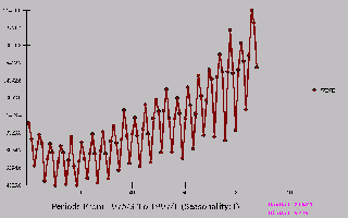
A plot of Wine against time illustrates a growth or trend. The data set is quarterly and evidences strong seasonal structure.

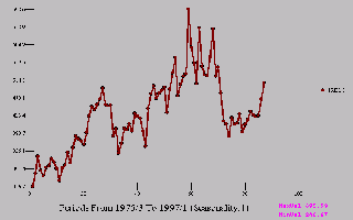
Italian Car Registrations has also grown over time.

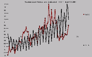
Plotting both series against time shows what appears to be association.

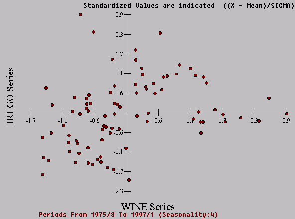
A scatter plot of Wine against Registrations confirms the association.

Simple cross-correlations use local means or averages as a filter.

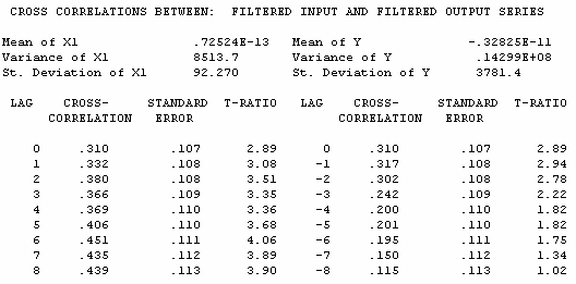
The cross-correlations indicate contemporaneous, i.e. instantaneous and lagged relationships between Wine and Registrations.

The regression model assumes an instaneous relationship is the correct one and that the error structure is uncorrelated. It would seem that there is a statistically significant relationship between these two series. This of course is spurious and caused by the common growth in these series caused by population growth. How to unmask and identify this spurious result is covered in the next few slides.

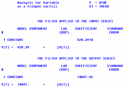
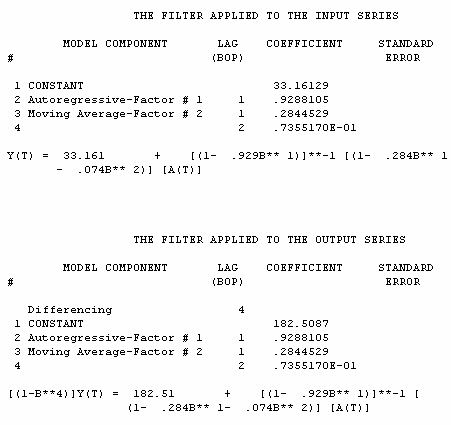
If we filter each of the two series using ARIMA structures we get:

We now use the ARIMA filter developed for the X series to eliminate the within relationship thus allowing a sharper view of the among relationship. In practice, we are converting an autocorrelated series (X) to an uncorrelated series for purposes of identifying significant cross-correlations.

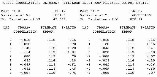
The cross-correlation pattern indicates that there is little or no incremental information in X.

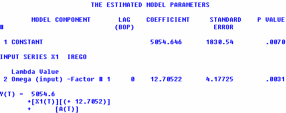
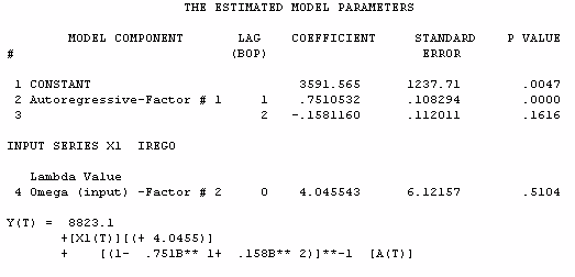
By estimating a combined regression and noise model, we find that the input series is not significant. We can then conclude that we have unmasked the spurious correlation between these two series. This combined regression/noise model is known as a Transfer Function or a Box-Jenkins model with a single endogenous (dependent) variable with one or more exogenous (input) series.

The data.

CLICK HERE:Home Page For AUTOBOX