Tom Reilly
Waging a war against how to model time series vs fitting
Build or Make your own ARIMA forecasting model?
- Font size: Larger Smaller
- Hits: 497801
- 0 Comments
- Subscribe to this entry
- Bookmark
It is the standard Economic Question. Should I make or build? The question here is: Should I build my own ARIMA modeling system or use software that can do this automatically? We lay out the general approach how to consider approaches to building a robust model. Easier said than done does apply here.
Overview
Autoregressive Integrated Moving Average (ARIMA) is a process designed to identify a weighted moving-average model specifically tailored to the individual dataset by using time series data to identify a suitable model. It is a rear-window approach that doesn’t use user-specified helping variables; such as price and promotion. It uses correlations within the history to identify patterns that can be statistically tested and then used to forecast. Often we are limited to using only the history and no causals whereas the general class of Box-Jenkins models can efficiently incorporate causal/exogenous variables (Transfer Functions or ARIMAX).
This post will introduce the steps and concepts used to identify the model, estimate the model, and perform diagnostic checking to revise the model. We will also list the assumptions and how to incorporate remedies when faced with potential violations.
Background
Our understanding of how to build an ARIMA model has grown since it was introduced in 1976 (1). Properly formed ARIMA models are a general class that includes all well-known models except some state space and multiplicative Holt-Winters models. As originally formulated, classical ARIMA modeling attempted to capture stochastic structure in the data; little was done about incorporating deterministic structure other than a possible constant and/or identifying change points in parameters or error variance.
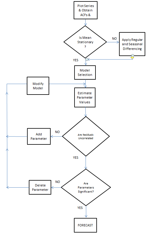
We will highlight procedures relevant to suggested augmentation strategies that were not part of the original ARIMA approach suggested in but are now standard. This step is often ignored as it is necessary that the mean of the residuals is invariant over time and that the variance of the final model’s errors is constant over time. Here is the classic circa 1970.
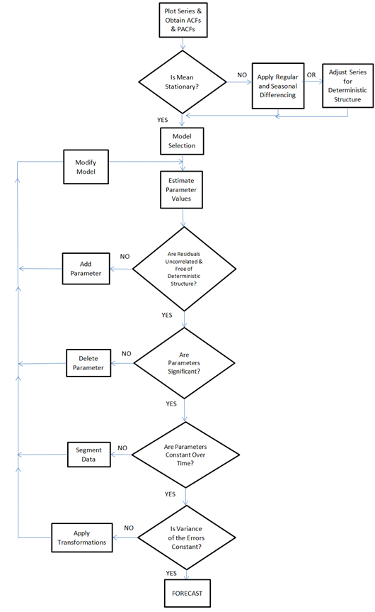
Here is the flowchart revised for additions by Tsay, Tiao, Bell, Reilly & Gregory Chow (ie chow test)
The idea of modeling is to characterize the pattern in the data and the goal is to identify an underlying model that is generating and influencing that pattern. The model that you will build should match the history which can then be extrapolated into the future. The actual minus the fitted values are called the residuals. The residuals should be random around zero (i.e. Gaussian) signifying that the pattern has been captured by the model.
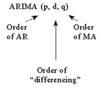
• For example, an AR model for monthly data may contain information from lag 12, lag 24, etc.
– i.e. Yt = A1Yt-12 +A2 Yt-24 + at
– This is referred to as an ARIMA(0,0,0)x(2,0,0)12 model
• General form is ARIMA(p,d,q)x(ps,ds,qs)s
Tools
The ARIMA process uses regression/correlation statistics to identify the stochastic patterns in the data. Regressions are run to find correlations based on different lags in the data. The correlation between successive months would be the lag 1 correlation or in ARIMA terms, the ACF of lag 1. We then examine if this month is related to one year ago at this time would then be apparent from evaluating the lag 12 correlation or in ARIMA terms, the ACF of lag 12. By studying the autocorrelations in the history, we can determine if there are any relationships and then take action by adding parameters to the model to account for that relationship. The different autocorrelations for the different lags are arranged together in what is known as a correlogram and are often presented using a plot. They are sometimes presented as a bar chart. We present it as a line chart showing 95% confidence limits around 0.0. The autocorrelation is referred to as the autocorrelation function (ACF).
- The key statistic in time series analysis is the autocorrelation coefficient (the correlation of the time series with itself, lagged 1, 2, or more periods).
The Partial Autocorrelation Function (PACF). The PACF of lag 12 for example is a regression using a lag of 12, but also uses all of the lags from 1 to 11 as well, hence the name partial. It is complex to compute and we won’t bother with that here.
Now that we have explained the ACF and the PACF, let’s discuss the components of ARIMA. There are three pieces to the model. The “I” means Integrated, but it simply means that you took differencing on the Y variable during the modeling process. The “AR” means that you have a model parameter that explicitly uses the history of the series. The “MA” means that you have a model parameter that explicitly uses the previous forecast errors. Not all models have all parts of the ARIMA model. All models can be re-expressed as pure AR models or pure MA models. The reason we attempt to mix and match has to do with attempting to use as few parameters as possible.
Identifying the order of differencing starts with the following initial assumptions, which are ultimately need to be verified:
1) The sequence of errors (a’s) are assumed to have a constant mean of zero and a constant variance for all sub-intervals of time.
2) The sequence of errors (a’s) are assumed to be normally distributed where the a’s are independent of each other.
3) Finally the model parameters and error variance are assumed to be fixed over all sub-intervals.
We study the ACF and PACF and identify an initial model. If this initial model is significant, the residuals will be free of structure and we are done. If not, we identify that structure and add it to the current model until a subsequent set of residuals is free of structure. One could consider this iterative approach as moving structure currently in the errors to the model until there is no structure in the errors to relocate.
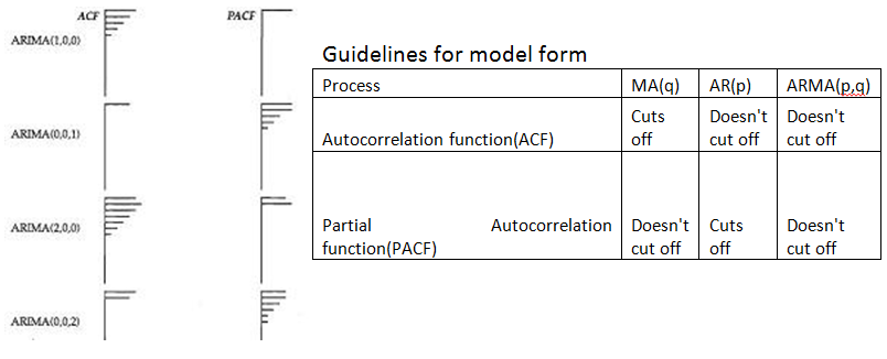
The following are some simplified guidelines to apply when identifying an appropriate ARIMA model with the following assumptions:
• Guideline 1: If the series has a large number of positive autocorrelations then differencing should be introduced. The order of the differencing is suggested by the significant spikes in the PACF based upon the standard deviation of the differenced series. This needs to be tempered with the understanding that a series with a mean change or a trend change can also have these characteristics.
• Guideline 2: Include a constant if your model has no differencing; include a constant elsewhere if it is statistically significant.
• Guideline 3: Domination of the ACF over the PACF suggests an AR model while the reverse suggests an MA model. The order of the model is suggested by the number of significant values in the subordinate.
• Guideline 4: Parsimony: Keep the model as simple as you can, but not too simple as overpopulation often leads to redundant structure.
• Guideline 5: Evaluate the statistical properties of the residual (at) series and identify the additional structure (step-forward) required
• Guideline 6: Reduce the model via step-down procedures to end up with a minimally sufficient model that has effectively deconstructed the original series to signal and noise. Over-differencing leads to unnecessary MA structure while under-differencing leads to overly complicated AR structure.
If a tentative model exhibits errors that have a mean change this can be remedied in a number of ways;
1) Identify the need to validate that the errors have constant mean via Intervention Detection (2,3) yielding pulse, seasonal pulse/level shift/local time trends
2) Confirming that the parameters of the model are constant over time
3) Confirming that the error variance has had no deterministic change points or stochastic change points.
The tool to identify omitted deterministic structure is fully explained in references 2 and 3 as follows:
1) use the model to generate residuals
2) identify the intervention variable needed following the procedure defined in reference
3) Re-estimate the residuals incorporating the effect into the model and then go back to Step 1 until no additional interventions are found.
Example 1) 36 annual values:
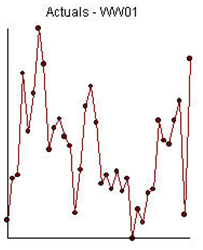
The ACF and the PACF suggest an AR(1) model (1,0,0)(0,0,0).
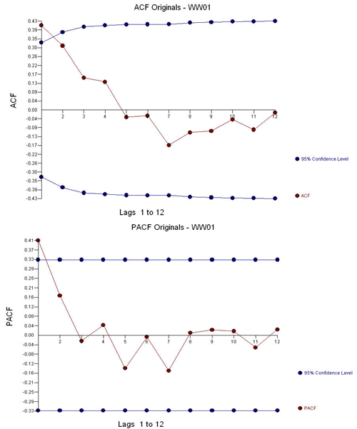
Leading to an estimated model (1,0,0)(0,0,0).

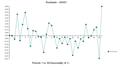
With the following residual plot, suggesting some “unusual values”:
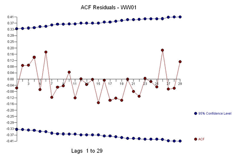
The ACF and PACF of the residuals suggests no stochastic structure as the anomalies effectively downward bias the results:
We added pulse outliers to create a more robust estimate of the ARIMA coefficients:

Example 2) 36 monthly observations:
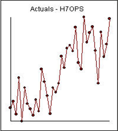
With ACF and PACF:
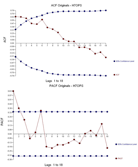
Leading to an estimated model: AR(2) (2,0,0)(0,0,0)

And with ACF of the residuals:
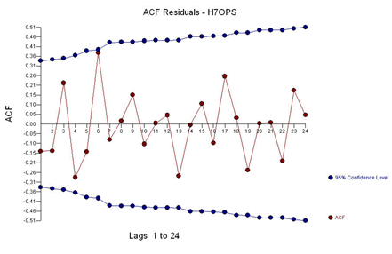
With the following residual plot:
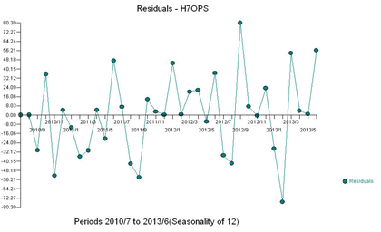
This example is a series that is better modeled with a step/level shift.
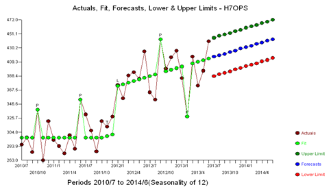
The plot of the residuals suggests a mean shift. Empowering Intervention Detection leads to an augmented model incorporating a level shift and a local time trend with and 4 pulses and a level shift. This model is as follows:

Example 3) 40 annual values:
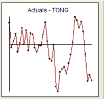
The ACF and PACF of the original series are:
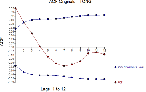
Suggesting a model (1,0,0,(0,0,0)

With a residual ACF of:
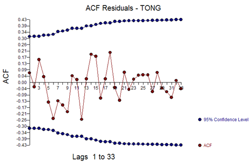
And residual plot:
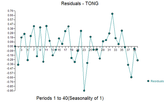
This suggests a change in the distribution of residuals in the second half of the time series. When the parameters were tested for constancy over time using the Chow Test (5), a significant difference was detected at period 21.

The model for period 1-20 is:

The model for period 21-40 is:

A final model using the last 20 values was:

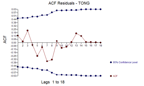
With residual ACF of:
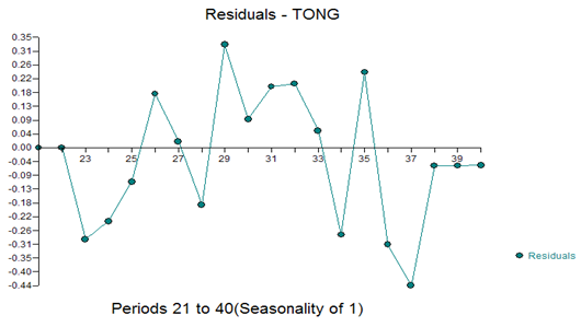
And residual plot of:
References
1)Box, G.E.P., and Jenkins, G.M. (1976). Time Series Analysis: Forecasting and Control, 2nd ed. San Francisco: Holden Day.
2)Chang, I., and Tiao, G.C. (1983). "Estimation of Time Series Parameters in the Presence of Outliers," Technical Report #8, Statistics Research Center, Graduate School of Business, University of Chicago, Chicago.
3)Tsay, R.S. (1986). "Time Series Model Specification in the Presence of Outliers," Journal of the American Statistical Society, Vol. 81, pp. 132-141.
4)Wei, W. (1989). Time Series Analysis Univariate and Multivariate Methods. Redwood City: Addison Wesley.
5)Chow, Gregory C. (1960). "Tests of Equality Between Sets of Coefficients in Two Linear Regressions". Econometrica 28 (3): 591–605
Comments
-
Please login first in order for you to submit comments
