Autobox Blog

Thoughts, ideas and detailed information on Forecasting.

  • Home
    Home This is where you can find all the blog posts throughout the site.
  • Categories
    Categories Displays a list of categories from this blog.
  • Tags
    Tags Displays a list of tags that has been used in the blog.
  • Bloggers
    Bloggers Search for your favorite blogger from this site.
Subscribe to this list via RSS Blog posts tagged in SAS forecasting arimax outliers sas transfer function hyndman

Alteryx is using the free "forecast" package in R. This BLOG is really more about the R forecast package then it is Alteryx, but since this is what they are offering.....

In their example on forecasting(they don't provide the data with Alteryx that they review, but you can request it---we did!), they have a video tutorial on analyzing monthly housing starts.

While this is only one example(we have done many!!).  They use over 20 years of data.  Kind of unnecessary to use that much data as patterns and models do change over time, but it only highlights a powerful feature of Autobox to protect you from this potential issue.  We will discuss down below the use of the Chow test.

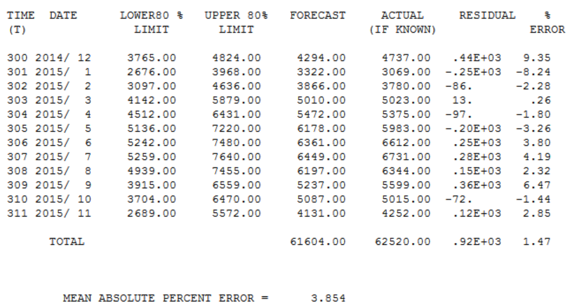
With 299 observations they determine of two alternative models (ie ETS and ARIMA)which the best model using the last 12 making a total of 311 observations used in the example. The video says they use 301 observations, but that is just a slight mistake.  It should be noted that Autobox doesn't ever withhold data as it has adaptive techniques which USE all of the data to detect changes.  It also doesn't fit models to data, but provides "a best answer".  Combinations of forecasts never consider outliers.  We do.

The MAPE for ARIMA was 5.17 and ETS was 5.65 which is shown in the video.  When running this in Autobox using the automatic mode, it had a 3.85 MAPE(go to the bottom). That's a big difference by improving accuracy by >25%.  Here is the model output and data file to reproduce this in Autobox.

Autobox is unique in that it checks if the model changes over time using the Chow test.  A break was identified at period 180 and the older data will be deleted.

      DIAGNOSTIC CHECK #4: THE CHOW PARAMETER CONSTANCY TEST
             The Critical value used for this test :     .01
             The minimum group or interval size was:     119

                    F TEST TO VERIFY CONSTANCY OF PARAMETERS                    
                                                                                
           CANDIDATE BREAKPOINT       F VALUE          P VALUE                  
                                                                                
               120 1999/ 12           4.55639          .0039929423              
               132 2000/ 12           7.41461          .0000906435              
               144 2001/ 12           8.56839          .0000199732              
               156 2002/ 12           9.32945          .0000074149              
               168 2003/ 12           7.55716          .0000751465              
               180 2004/ 12           9.19764          .0000087995*             

* INDICATES THE MOST RECENT SIGNIFICANT  BREAK POINT:    1% SIGNIFICANCE LEVEL. 

  IMPLEMENTING THE BREAKPOINT AT TIME PERIOD    180: 2004/   12 

  THUS WE WILL DROP (DELETE) THE FIRST   179 OBSOLETE OBSERVATIONS
  AND ANALYZE THE MOST RECENT   120 STATISTICALLY HOMOGENOUS OBSERVATIONS


DIAGNOSTIC CHECK #4: THE CHOW PARAMETER CONSTANCY TEST The Critical value used for this test : .01 The minimum group or interval size was: 119 F TEST TO VERIFY CONSTANCY OF PARAMETERS CANDIDATE BREAKPOINT F VALUE P VALUE 120 1999/ 12 4.55639 .0039929423 132 2000/ 12 7.41461 .0000906435 144 2001/ 12 8.56839 .0000199732 156 2002/ 12 9.32945 .0000074149 168 2003/ 12 7.55716 .0000751465 180 2004/ 12 9.19764 .0000087995* * INDICATES THE MOST RECENT SIGNIFICANT BREAK POINT: 1% SIGNIFICANCE LEVEL.

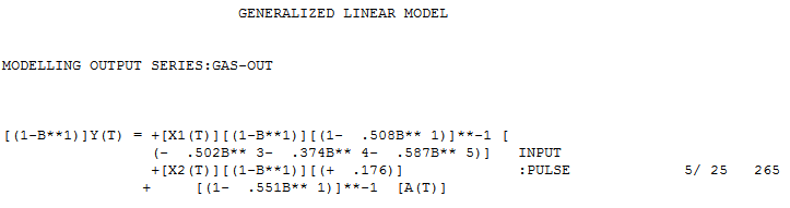
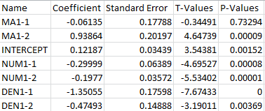
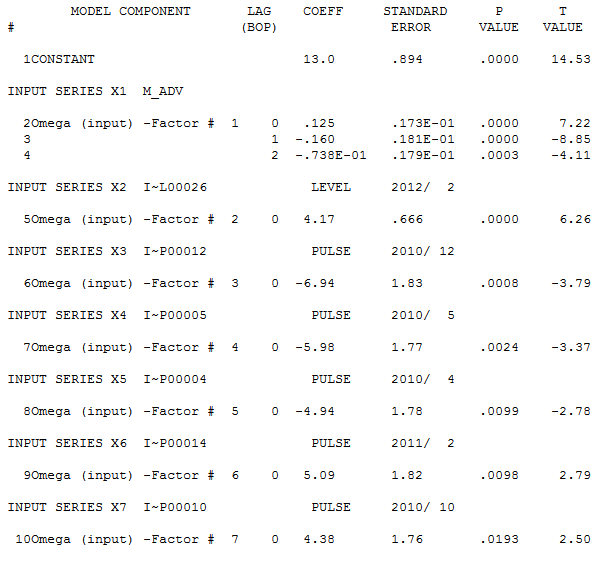
The model built using the more recent data had seasonal and regular differencing, an AR1 and a weak AR12.  Two outliers were found at period 225(9/08) and 247(7/10).  If you look at September's they are typically low, but not in 2008. July's are usually high, but not in 2010.  If you don't identify and adjust for these outliers then you can never achieve a better model.  Here is the Autobox model                                                                                                               

[(1-B**1)][(1-B**12)]Y(T) =                                                                                   
         +[X1(T)][(1-B**1)][(1-B**12)][(-  831.26    )]       :PULSE          2010/  7   247
         +[X2(T)][(1-B**1)][(1-B**12)][(+  613.63    )]       :PULSE          2008/  9   225
        +     [(1+  .302B** 1)(1+  .359B** 12)]**-1  [A(T)]

Alteryx ends up using an extremely convoluted model.  An ARIMA(2,0,2)(0,1,2)[12] with no outliers. That is a whopping 6 parameters vs Autobox's 2 parameters.

Let's take a look at the residuals. It tells everything you need to know.  Period 200 to 235 the model is overfitting the data causing there to be a large are mismodeled. Remember that Autobox found a break at period 180 which is close to period 200. The high negative error(low residual) is the July 2010 outlier that Autobox identifies.  If you ignore outliers they play havoc with your model.


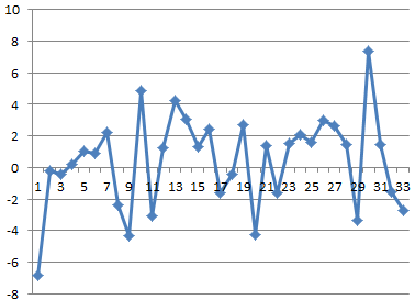
Here is the table for forecasts for the 12 withheld periods.


Posted by on in Forecasting

In 2011, IBM Watson shook our world when it beat Ken Jennings on Jeopardy and "Computer beats Man" was the reality we needed to accept.


IBM's WatsonAnalytics is now avalilabe for a 30 day trial and it did not shake my world when it came to time series analysis.  They have a free trial to download and play with the tool. You just need to create a spreadsheet with a header record with a name and the data below in a column and then upload the data very easily into the web based tool.


It took two example time series for me to wring my hands and say in my head, "Man beats Computer".  Sherlock Holmes said, "It's Elementary my dear Watson".  I can say, "It is not Elementary Watson and requires more than pure number crunching using NN or whatever they have".


The first example is our classic time series 1,9,1,9,1,9,1,5 to see if Watson could identify the change in the pattern and mark it as an outlier(ie inlier) and continue to forecast 1,9,1,9, etc.  It did not.  In fact, it expected a causal variable to be present so I take it that Watson is not able to handle Univariate problems, but if anyone else knows differently please let me know.


The second example was originally presented in the 1970 Box-Jenkin's text book and is a causal problem referred to as "Gas Furnace" and is described in detail in the textbook and also on NIST.GOV's website.  Methane is the X variable and Y is the Carbon Dioxide output.  If you know or now closely examine the model on the NIST website, you will see a complicated relationship where there is a complicated relationship between X and Y that occurs with a delay between the impact of X and the effect on Y (see Yt-1 and Yt-2 and Xt-1 and Xt-2 in the equation).  Note that the R Squared is above 99.4%!  Autobox is able to model this complex relationship uniquely and automatically.  Try it out for yourself here! The GASX problem can be found in the "BOXJ" folder which comes with every installed version of Autobox for Windows.

Watson did not find this relationship and offered a predictive strength of only 27%(see the X on the left hand of the graph) compared to 96.4%.  Not very good. This is why we benchmark. Please try this yourself and let me know if you see something different here.


gasx watson


Autobox's model has lags in Y and lags in the X from 0 to 7 periods and finds an outlier(which can occur even in simulated data out of randomness).  We show you the model output here in a "regression" model format so it can be understood more easily. We will present the Box-Jenkins version down below.

gasx rhs


Here is a more parsimonious version of the Autobox model in pure Box-Jenkins notation.  Another twist is that Autobox found that the variance increased at period 185 and used Weighted Least Squares to do the analysis hence you will see the words "General Linear Model" at the top of the report.


gasx


It's been 6 months since ourlast BLOG.  We have been very busy.


We engaged in a debate on a linkedin discussion group over the need to pre-screen your data so that your forecasting algorithm can either apply seasonal models or not consider seasonal models.  A set of GUARANTEED random data was generated and given to us as a challenge four years ago.  This time we looked a little closer at the data and found something interesting. 1)you don't need to pres-creen your data 2)be careful how you generate random data


Here is my first response:

As for your random data, we still have it when you send it 4 years ago. I am not sure what you and Dave looked at, but if you download run the 30 day trial now and we always have kept improving the software you will get a different answer and the results posted here on dropbox.com.https://www.dropbox.com/s/s63kxrkquzc6e00/output_miket.zip

I have provided your data(xls file),our model equation (equ), forecasts(pro), graph(png) and audit of the model building process(htm).

Out of the 18 examples, Autobox found 6 with a flat forecast, 7 with 1 monthly seasonal pulse or a 1 month fixed effect, 4 with 2 months that had a mix of either a seasonal pulse or a 1 month fixed effect, 2 with 3 months that had a mix of either a seasonal pulses or a 1 month fixed effect.

Note that no model was found with Seasonal Differencing, AR12, with all 11 seasonal dummies.

Now, in a perfect world, Autobox would have found 19 flat lines based on this theoretical data. If you look at the data, you will see that there were patterns found where Autobox found them that make sense. There are sometimes seasonality that is not persistent and just a couple of months through the year.

If we review the 12 series where Autobox detected seasonality, it is very clear that in the 11 of the 12 cases that it was justified in doing so. That would make 17 of the 18 properly modeled and forecasted.

Series 1 - Autobox found feb to be low. A All three years this was the case. Let's call this a win.

Series 2 - Autobox found apr to be low. All three years were low. Let's that call this a win.

Series 3- Autobox found sep and oct to be low. 4 of the 6 were low and the four most recent were all low supporting a change in the seasonality. Let's call this a win.

Series 4- Autobox found nov to be low. All three years were low. Let's call this a win.

Series 5- Autobox found mar, may and aug to be low. All three years were low. Let's call that a win.

Series 7- Autobox found jun low and aug high. All three years matched the pattern. Let's call that a win.

Series 10 - Autobox found apr and jun to be high. 5 of the 6 data points were high. Let's call this a win.

Series 12 - Autobox found oct to be high and dec to be low. All three years this was the case. Let's call this a win.

Series 13 - Autobox found aug to be high. Two of the three years were very very high. Let's call this a win.

Series 14 - Autobox found feb and apr to be high. All three years this was the case. Let's call this a win.

Series 15 - Autobox found may jun to be high and oct low. 8 of the 9 historical data points support this, Let's call this a win.

Series 16 - Autobox found jan to below. It was very low for two, but one was quite high and Autobox called that an outlier. Let's call this a loss.

A little sleep and then I posted this response:

After sleeping on that very fun excercise, there was something that still wasn't sitting right with me. The "guaranteed" no seasonality statement didn't match with the graph of the datasets. They didn't seem to have randomness and seemed more to have some pattern.

I generated 4 example datasets from the link below. I used the defaults and graphed them. They exhibited randomness. I ran them through Autobox and all had zero seasonality and flat forecasts.

http://www.random.org/sequences/


We got into an interesting debate on model performance on a classic time series that has been modeled in the famous textbooks and we tried it out on some very expensive statistical software. It's tough to find a journal that is willing to criticize its main advertiser so we will do it for them. The time series is Sales and Advertising and you can even download down below and do this with your own forecasting/modeling tool to see what it does!  Feel free to post your results and continue the debate of what is a good model!

What ingredients are needed in a model?    We have two modeling violations that seem to be ignored in this example:

1)Skipping Identification and "fitting" based on some AIC criteria. Earlier researchers would restrict themselves to lags of y and lags of X and voila they had their model.

2)Ignoring Modern day remedies, but not all do this.  Let's list them out 1)Outliers such as pulses, level shifts, time trends and seasonal pulses.  The historical data seems to exhibit an increasing trend or level shift using just your eyes and the graph. 2)Dealing with too many observations as the model parameters have changed over time(ie Chow test) 3)Dealing with non-constant variance.  These last two don't occur in our example so don't worry about them right now.

Are you (or by default your software) using dated methods to build its regression model?  Is it leaning on the AIC to help build your regression using high order lags?  Said more clearly,  “Are you relying upon using long lags of X in a regression and ignoring using Stochastic (ie ARIMA) or deterministic empirically identified variables to build your model?”   Are you doing this and doing it automatically and potentially missing the point of how to properly model?  Worse yet, do your residuals look like they fail the random (ie N.I.I.D) tests with plots against time?  The annointed D-W statistic can be flawed if there are omitted dummy variables needed such as level shifts, pulses, time trends, or seasonal pulses.  Furthermore, D-W ignores lags 2 and out which ignores the full picture.

See the flow chart on the right hand side on the link in the next sentence. A good model has been tested for necessity and sufficiency. It has also been tested for randomness in the errors.

While it is easy and convenient (and makes for quick run time) to use long lags on X, it can often be insufficient and presumptory (see Model Specification Bias) and leave an artifact in the residuals suggesting an insufficient model.

Regression modelers already know about necessity and sufficiency tests, but users of fancy software don't typically know these important details as to how the system got the model and perhaps a dangerous one?  Necessity tests question whether the coefficients in your model are statistically significant (ie not needed or "stepdown").  Sufficiency tests question whether the model is missing variables and therefore ruled as insufficient(ie need to add more variables or "stepup").

Is it possible for a model to fail both of these two critical tests at the same time?Yes.

Let's look at an example. If we have a model where Y is related to X and previous of values of X up to lag and including lag 4, and lags 2, 3 and 4 are not significant then they should be deleted from the model.  If you don’t remove lag 2, 3 and 4 then you have failed the necessity test and you model is suboptimal.  Sounds like the stepdown step has been bypassed? Yes. The residuals from the “overpopulated” model could(and do!) have pulses and a level shift in the residuals ignored and therefore an insufficient model.

Let’s consider the famous dataset of Sales and Advertising from Blattberg and Jeuland in 1981 that has been enshrined into textbooks like Makradakis, Hyndman and Wheelwright 3rd edition.  See pages 411-413  for this example in the book. The data is 3 years of monthly data.

http://mansci.journal.informs.org/content/27/9/988.full.pdf

Sales - 12,20.5,21,15.5,15.3,23.5,24.5,21.3,23.5,28,24,15.5,17.3,25.3,25,36.5,36.5,29.6,30.5,28,26,21.5,19.7,19,16,20.7,26.5,30.6,32.3,29.5,28.3,31.3,32.2,26.4,23.4,16.4

Adv - 15,16,18,27,21,49,21,22,28,36,40,3,21,29,62,65,46,44,33,62,22,12,24,3,5,14,36,40,49,7,52,65,17,5,17,1

The model in the textbook has 3 lags that are not significant and thereby not sufficient. The errors from the model show the need for AR1 when one is not needed of course due to the fact that there is a poor model being used.  The errors are not random and exhibit a level shift that is not rectified.

In 2013, the largest company that offers statistical software (and very expensive) is seemingly inadequate.  We will withhold the name of this company. The Emperor has no clothes? Nope. She does not. Here is the model in the textbook estimated in Excel (which can be reproduced in Autobox).  The results in the textbook are about the same as this output.  You can clearly see that lags 3,4,5 are NOT SIGNIFICANT, right? Does that bother you?

The residuals are not random and exhibit a level shift in the second half of the data set and two big outliers in the first half not addressed.


Ok, here is the fat and happy expensive forecasting system results (ie "fatted calf" so to speak).  Do you get results like this?  If you did, then you paid too much and got too little.

The MA's 1st parameter was not significant, but kept in the model.  This is indicative of an overparameterized model.  The overloading of coefficients without efficient identification has consequences.


Lack of due diligence - No effort is being made to consider deterministic violations of the error terms.  There are two outliers (one at the beginning and one at the end that are very large (ie 8)) and are not being dealt with which impacts the model/forecast that has been built.

Autobox's turn - Classical remedies have been to add all lags from 0 to N as compared to a smarter approach where only significant variables that also reacts to structure in the errors which could be both stochastic and deterministic.  All the parameters are significant.  Only numerator parameters were needed and no denominator. Note: Stochastic being ARMA structure and deterministic being dummy variables such as pulses, level shifts, time trends and seasonal pulses.

Here are the residuals which are free of pattern.  The last value is ok(ie ~4), but could be confused to be an outlier, but in the end everything is an outlier. :)


If you don’t have the ammunition to examine the errors with a close eye you end up with a model that can fail both necessity and sufficiency at the same time.

Leaning on the AIC leads to ignoring necessity, sufficiency and nonrandom errors and bad models.

Some models in text books show bad models and the keep the modeling approach as simple as possible and are in fact doing damage to the student.  When students become practitioners they find that the text book approach just doesn’t work.


Go to top